I don't normally do follow-ups and never this quick. After posting that last article, it was fun to read the comments on Reddit and Hacker News as they rolled in. I even found other discussions. I couldn't help wonder, "Could I have made it even more performant?". After heading home I decided to take another look.

There was.

 

Gotta Go Fast

Look at the implementation of the Cg asin() approximation;

double asin_cg(const double x)
{
    // Original Minimax coefficients
    constexpr double a0 = 1.5707288;
    constexpr double a1 = -0.2121144;
    constexpr double a2 = 0.0742610;
    constexpr double a3 = -0.0187293;

    // Strip sign
    const double abs_x = abs(x);

    // Evaluate polynomial using Horner's method
    double p = a3 * abs_x + a2;
    p = p * abs_x + a1;
    p = p * abs_x + a0;

    // Apply sqrt term and pi/2 offset
    const auto x_diff = sqrt(1.0 - abs_x);
    const double result = (Pi / 2.0) - (x_diff * p);

    // Restore sign natively
    return copysign(result, x);
}

 

Does something about how p is computed look a little curious? It can be rewritten to be fully const. While it's not a requirement, it's generally something you should strive for. This was missed in the first pass.

const double p = ((a3 * abs_x + a2) * abs_x + a1) * abs_x + a0;

 

From here we can do a polynomial expansion and factoring. This is where the magic happens. Showing the work step by step: \

p = ((a3 * abs_x + a2) * abs_x + a1) * abs_x + a0
p = (a3 * abs_x * abs_x + a2 * abs_x + a1) * abs_x + a0
p = (a3 * abs_x^2 + a2 * abs_x + a1) * abs_x + a0
p = a3 * abs_x^3 + a2 * abs_x^2 + a1 * abs_x + a0
p = (a3 * abs_x^3 + a2 * abs_x^2) + (a1 * abs_x + a0)
p = (a3 * abs_x + a2) * abs_x^2 + (a1 * abs_x + a0)

 

Taking that last term for p, we have this in code:

const double x2 = abs_x * abs_x;
const double p = (a3 * abs_x + a2) * x2 + (a1 * abs_x + a0);

(full function available here)

 

p is now evaluated a little bit differently but arrives at the same numerical value. We are now leveraging a technique known as Estrin's Scheme to rewrite this equation. With the above, the compiler (and CPU) can evaluate a3 * abs_x + a2 and a1 * abs_x + a0 independently of each other. This reduces the dependency chain length from three to two, allowing modern out-of-order CPUs to execute these operations in parallel. For those unaware, this is Instruction-level parallelism.

 

Benchmark Measurements

The full benchmarking code is available here. This gets into microbenchmarking (a little bit), which is fairly tricky. A full "run" of the benchmark has 10,000,000 calls to the respective arcsine function, and each chip/OS/compiler combo does 250 runs in total. Testing environments were:

• Intel i7-10750H
  • Ubuntu 24.04 LTS: GCC & clang
  • Windows 11: GCC & MSVC
• AMD Ryzen 9 6900HX
  • Ubuntu 24.04 LTS: GCC & clang
  • Windows 11: GCC & MSVC
• Apple M4
  • macOS Tahoe: GCC & clang

 

I'd love to measure this on some mobile chips and a newer Intel, but this is what I own. Gifts are always welcome.  The data is as follows (and details are here if you're interested). A lower ms count is the most desirable and std::asin() is the baseline.

Intel Core i7
  Linux
    GCC 14.2 (-O3)
      std::asin()         :  74385 ms
      asin_cg()           :  48374 ms -- 1.54x
      asin_cg_estrin()    :  41388 ms -- 1.80x
    Clang 20.1 (-O3)
      std::asin()         :  73504 ms
      asin_cg()           :  47211 ms -- 1.56x
      asin_cg_estrin()    :  41350 ms -- 1.78x
  Windows
    GCC 14.2 (-O3)
      std::asin()         : 113396 ms
      asin_cg()           :  91925 ms -- 1.23x
      asin_cg_estrin()    :  90925 ms -- 1.25x
    MSVC VS 2022 (/O2)
      std::asin()         :  84733 ms
      asin_cg()           :  53592 ms -- 1.58x
      asin_cg_estrin()    :  45014 ms -- 1.88x

AMD Ryzen 9
  Linux
    GCC 14.2 (-O3)
      std::asin()         :  74986 ms
      asin_cg()           :  53129 ms -- 1.41x
      asin_cg_estrin()    :  52166 ms -- 1.44x
    Clang 20.1 (-O3)
      std::asin()         :  75188 ms
      asin_cg()           :  52837 ms -- 1.42x
      asin_cg_estrin()    :  51856 ms -- 1.45x
  Windows
    GCC 14.2 (-O3)
      std::asin()         : 136393 ms
      asin_cg()           : 122071 ms -- 1.12x
      asin_cg_estrin()    : 120953 ms -- 1.13x
    MSVC VS 2022 (/O2)
      std::asin()         : 121639 ms
      asin_cg()           :  92612 ms -- 1.31x
      asin_cg_estrin()    :  92290 ms -- 1.32x

Apple M4
  macOS
    GCC 15.1.0 (-O3)
      std::asin()         :  26176 ms
      asin_cg()           :  25764 ms -- 1.02x
      asin_cg_estrin()    :  25668 ms -- 1.02x
    Apple Clang 17.0.0 (-O3)
      std::asin()         :  33626 ms 
      asin_cg()           :  32755 ms -- 1.03x
      asin_cg_estrin()    :  30245 ms -- 1.11x

 

Summarizing the above:

• AMD has barely any speedup. So it does not help, but it doesn't hurt either
• The (older) Intel chip gets a massive boost using the Estrin method of the Cg version (Windows/GCC excluded)
• The speedup on Apple's Chip is only present when compiling with clang
  • But GCC's code is faster

 

Ray Tracer Measurements

I'll use the same test as the last article. Taking a few renders, this is what a median run looked like. On Intel i7, using the older asin_cg() method:

ben@linux:~/Projects/PSRayTracing/build_gcc_14$ ./PSRayTracing -n 250 -j 4 -s 1920x1080
Scene: book2::final_scene
Render size: 1920x1080
Samples per pixel: 250
Max number of ray bounces: 50
Number of render threads: 4
  Copy per thread: on
Saving to: render.png
Seed: `ASDF`
Rendering: [==================================================] 100% 212s
Render took 212.311 seconds

 

Turning on this new Estrin optimization:

ben@linux:~/Projects/PSRayTracing/build_gcc_14$ ./PSRayTracing -n 250 -j 4 -s 1920x1080
...
Rendering: [==================================================] 100% 206s
Render took 205.99 seconds

 

A nice +3% speedup over the asin_cg() method from last time. We're not going to see a massive jump like the benchmark above since calling arcsine is such a small part of this program (compared to everything else). On the Apple M4 Mac Mini (Tahoe), with the old asin_cg():

ben@Mac build_clang_17 % ./PSRayTracing -j 4 -n 250 -s 1920x1080
...
Render took 101.747 seconds

 

Plugging in our new one:

ben@Mac build_clang_17_asin_cg_estrin % ./PSRayTracing -n 250 -s 1920x1080 -j 4
Render took 101.817 seconds

 

While on the surface this might look like an absolutely atomic performance degradation, it's actually nothing. Rendering each time can vary give or take two seconds, despite the ray tracer being fully deterministic. I usually chalk this up to "gremlins in the computer" and by that, I mean things like the OS doing context switching and CPUs having dynamic clocks. The best thing to do would be to take 250 runs of this. I don't think it's worth it. From a heuristic standpoint 0.1 seconds is not a lot of time out of 102. Also clang on the M4 doesn't have that much of a speedup when doing asin_cg_estrin() vs the plain asin_cg().

 

Last Words (and Opinions)

When I started work on PSRayTracing, I wanted to show off how you can rewrite your code for the compiler to make better optimizations; this is another one of them. In this series I hope I've really hammered down the importance of benchmarking (i.e. taking measurements) as well. This is something I do not see others doing.

I took a brief look at using a LUT, while that might have been faster in the past (and on paper), it wasn't the case for me. It also had a lot more error. Email me for charts. Stick with a math formula. It's simpler. Using SIMD to speed up the computation isn't an option either due to the architecture of the original code PSRayTracing was based on. It's something I'd like to do, as sometimes a performance bottleneck can be architectural, but there are many other ways I'd like to spend my days in this life.

Lastly, keep in mind this is an approximation of arcsine, not the actual method. Most of the time (especially for computer graphics) you can get away with one, but there are cases where you cannot.

Always step back from the problem, collaborate, and then reevaluate. You'll find something better.

This one is going to be a quick one as there wasn't anything new discovered. In fact, I feel quite dumb. This is really a tale of "Do your research before acting and know what your goal is," as you'll end up saving yourself a lot of time. Nobody likes throwing away work they've done either, and there could be something here that is valuable for someone else.

---

I still can't escape PSRayTracing. No matter how hard I try to shelve that project, every once in a while I hear about something "new" and then wonder "can I shove this into the ray tracer and wring a few more seconds of speed out of it?" This time around it was Padé Approximants. The target is to provide me with faster (and better) trig approximations.

Short answer: "no". It did not help.

But... I found something that ended up making the ray tracer significantly faster!!

 

Quicker Trig

In any graphics application trigonometric functions are frequently used. But that can be a little expensive in terms of computational time. While it's nice to be accurate, we usually care more about fast if anything. So if we can find an approximation that's "good enough" and is speedier than the real thing, it's generally okay to use it instead.

When it comes to texturing objects in PSRayTracing (which is based off of the Ray Tracing in One Weekend books, circa the 2020 edition), the std::asin() function is used. When profiling some of the scenes, I noticed that a significant amount of calls were made to that function, so I thought it was worth trying to find an approximation.

In the end I ended up writing my own Taylor series based approximation. It is faster but also has a flaw, whenever the input x was less than -0.8 or greater than 0.8 it would deviate heavily. So to look correct, it had to fall back to std::asin() past these bounds.

 

The C++ is as follows:

double _asin_approx_private(const double x)
{
    // This uses a Taylor series approximation.
    // See: http://mathforum.org/library/drmath/view/54137.html
    //
    // In the case where x=[-1, -0.8) or (0.8, 1.0] there is unfortunately a lot of
    // error compared to actual arcsin, so for this case we actually use the real function
    if ((x < -0.8) || (x > 0.8))
    {
        return std::asin(x);
    }

    // The taylor series approximation
    constexpr double a = 0.5;
    constexpr double b = a * 0.75;
    constexpr double c = b * (5.0 / 6.0);
    constexpr double d = c * (7.0 / 8.0);

    const double aa = (x * x * x) / 3.0;
    const double bb = (x * x * x * x * x) / 5.0;
    const double cc = (x * x * x * x * x * x * x) / 7.0;
    const double dd = (x * x * x * x * x * x * x * x * x) / 9.0;

    return x + (a * aa) + (b * bb) + (c * cc) + (d * dd);
}

 

After a bit of trial and error, I found that a fourth-order Taylor series was the most performant on my hardware. It was measurably faster (by +5%), so I kept it and moved onto the next optimization.

 

Padé Approximants

I can't remember where I heard about this one.... I'm drawing a complete blank. If you want a more in depth read, check the Wikipedia article. But in a quick nutshell, they are a mathematical tool they can help provide an approximation of an existing function. To compute one, you do need to start out with a Taylor (or Maclaurin) series. While PSRayTracing is mainly a C++ project, Python is going to be used for simplicity's sake; we'll go back to our favorite compiled language when it matters though.

For the arcsine approximation above, using the four-term Taylor, we have this in Python:

def taylor_fourth_order(x: float) -> float:
    return x + (x**3)/6 + (3*x**5)/40 + (5*x**7)/112

 

Computing that into a Padé Approximant, we get what's known as a [3/4] Padé Approximant:

def asin_pade_3_4(x):
    a1 = -367.0 / 714.0
    b1 = -81.0 / 119.0
    b2 = 183.0 / 4760.0
    n = 1.0 + (a1 * x**2)
    d = 1.0 + (b1 * x**2) + (b2 * x**4)
    return x * (n / d)

 

I'm also going to provide the one from a 5th order Taylor Series as well, a [5/4] Padé Approximant:

def asin_pade_5_4(x):
    a1 = -1709.0 / 2196.0
    a2 =  69049.0 / 922320.0
    b1 = -2075.0 / 2196.0
    b2 =  1075.0 / 6832.0
    n = 1.0 + (a1 * x**2) + (a2 * x**4)
    d = 1.0 + (b1 * x**2) + (b2 * x**4)
    return x * (n / d)

 

Now when charting all three, we get this:

 

Wow, that already looks much better. Less error! It's a bit hard to see that, so let's zoom in on right side of the functions:

 

The error hasn't fully gone away, but it's much less than before. Instead of defaulting back to the built-in asin() method, there's a better trick up our sleeves: leveraging Inverse Trig Functions/Half Angle Transforms. Look at this:

This does seem a tad confusing, yet it lets us do a pro gamer move. When |x| is past a value we can "teleport" from the edge of the function more towards the center of arcsin(), perform the computation, and then go back and use the result there. In Python, this is our new asin(x) approximation:

def asin_pade_3_4_half_angle_correction(x: float) -> float:
    abs_x = abs(x)

    # If past the range, then we can use the half angle transformation to account for error
    if abs_x > 0.85:
        small_x = math.sqrt(0.5 * (1.0 - abs_x))
        r = (math.pi / 2) - (2.0 * asin_pade_3_4(small_x))
        return -r if x < 0 else r

    # Within the border we can just use the 3/4 approximation like normal
    return asin_pade_3_4(x)

 

Now with the correction in place, the edges look more like this:

 

It might be a little hard to see, but the dashed lines are the ones with this half angle transform correction method and they are hugging the y=0 line. There is a tiny bit of error if you zoom in.

There's even a further optimization that could be had: use (and adapt) a [1/2] Padé on the inside of the if body. This is because small_x will always be less than the square root of 0.075 (which is ~0.27). The [1/2] Padé approximant for asin() can compute much faster, but only for smaller values of x. It can even be inlined into our function for further optimization. See below:

def asin_pade_1_2(x):
    b1 = -1.0 / 6.0
    d = 1.0 + (b1 * x**2)
    return (x / d)

# ...

def asin_pade_3_4_half_angle_correction(x: float) -> float:
    abs_x = abs(x)

    # If past the range, then we can use the half angle transformation to account for error along with a "smaller" Pade
    if abs_x > 0.85:
        z = (1.0 - abs_x) / 2
        b1 = -1.0 / 6.0
        d = 1.0 + (b1 * z)
        small_pade = math.sqrt(z) / d
        r = (math.pi / 2) - (2.0 * small_pade)
        return -r if x < 0 else r

    # Within the border we can just use the 3/4 approximation like normal
    return asin_pade_3_4(x)

 

It still looks the same as the above chart, so I don't think it's necessary to include another one. Written as C++, we have this:

constexpr double HalfPi = 1.5707963267948966;

inline double asin_pade_3_4(const double x)
{
   constexpr double a1 = -367.0 / 714.0;
   constexpr double b1 = -81.0 / 119.0;
   constexpr double b2 = 183.0 / 4760.0;

   const double x2 = x * x;
   const double n = 1.0 + (a1 * x2);
   const double d = 1.0 + (b1 * x2) + (b2 * x2 * x2);

   return x * (n / d);
}

double asin_pade_3_4_half_angle_correction(const double x)
{
   const double abs_x = std::abs(x);

   if (abs_x <= 0.85)
   {
       return asin_pade_3_4(x);
   }
   else
   {
       // Edges of Pade curve
       const double z = 0.5 * (1.0 - abs_x);
       constexpr double b1 = -1.0 / 6.0;
       const double d = 1.0 + (b1 * z);
       const double pade_result = std::sqrt(z) / d;
       const double r = HalfPi - (2.0 * pade_result);
       return std::copysign(r, x);
   }
}

 

Compared to the original approximation method, this is more complicated, but it has benefits:

1. For a larger range [-0.85, 0.85] it will default to a simpler computation
2. For the edge cases it will use a quicker computation than std::asin()
3. There is less error

I'm very much a "put up or shut up" type of person. So let's actually plug it back into PSRayTracing and see if there is a speed improvement. We'll use the default scene (which is the final render from book 2):

 

Measuring

That globe is the user of asin(). All images generally look the same (minus a little fuzz). For the test case we will render a 1080p image, with 250 samples per pixel, and take up a few cores. The testing was done on an M4 Mac Mini (running a version of macOS Tahoe, using GCC15 compiled with -O3). Doing a few runs each, taking a median:

With std::asin() it took about 111 seconds to render the scene:

ben@Benjamins-Mac-mini build_gcc15 % ./PSRayTracing -j 4 -n 250 -s 1920x1080 -o render_std_asin.png
Scene: book2::final_scene
Render size: 1920x1080
Samples per pixel: 250
Max number of ray bounces: 50
Number of render threads: 4
  Copy per thread: on
Saving to: render_std_asin.png
Seed: `ASDF`
Rendering: [==================================================] 100% 111s
Render took 110.891 seconds

 

The older asin() approximation took roughly 105 seconds (~5% speedup):

ben@Benjamins-Mac-mini build_gcc15 % ./PSRayTracing -j 4 -n 250 -s 1920x1080 - o render_asin_taylor.png
...
Render took 104.674 seconds

 

And this new Padé Approximant approach took... The same amount of time:

ben@Benjamins-Mac-mini build_gcc_15 % ./PSRayTracing -j 4 -n 250 -s 1920x1080 -o render_asin_pade.png
...
Render took 104.87 seconds

 

This new asin() method is better (in terms of correctness), but not much of a contest when it comes to performance. It's a small victory.

 

An LLM Prompt

There's no denying the AI tooling of the past 3+ years is going to go away. At CppCon 2023 Andrei Alexandrescu gave an excellent talk entitled "Robots Are After Your Job: Exploring Generative AI for C++"; it's worth your time to listen. After all of the above work and that talk in mind, I decided to ask an LLM (Gemini in this case): "What's a fast approximation for asin(x) I can use in C++?". It gave me this:

constexpr double HalfPi = 3.1415926535897932385 / 2.0;

double fast_asin_cg(const double x)
{
    // Original Minimax coefficients
    constexpr double a0 =  1.5707288;
    constexpr double a1 = -0.2121144;
    constexpr double a2 =  0.0742610;
    constexpr double a3 = -0.0187293;

    // Strip sign
    const double abs_x = fabs(x);

    // Evaluate polynomial using Horner's method
    double p = a3 * abs_x + a2;
    p = p * abs_x + a1;
    p = p * abs_x + a0;

    // Apply sqrt term and pi/2 offset
    const double x_diff = sqrt(1.0 - abs_x);
    const double result = HalfPi - (x_diff * p);

    // Restore sign
    return copysign(result, x);
}

 

This looked too simple for me to believe. The source it cited was the documentation for asin in Nvidia's Cg Toolkit; a product that hasn't been updated since 2012. The reference implementation contained a rewritten form of the above. Porting it over to Python/Jupyter to verify it is trivial:

def asin_cg(x: float) -> float:
    '''
    Fast branchless asin(x) approximation.
    Based on Abramowitz and Stegun formula 4.4.45
    '''
    # https://developer.download.nvidia.com/cg/asin.html
    # https://personal.math.ubc.ca/~cbm/aands/page_81.htm

    # Original Minimax coefficients from Abramowitz and Stegun
    a0 =  1.5707288
    a1 = -0.2121144
    a2 =  0.0742610
    a3 = -0.0187293

    abs_x = abs(x)

    # Evaluate polynomial using Horner's method
    p = a3 * abs_x + a2
    p = p * abs_x + a1
    p = p * abs_x + a0

    result = (math.pi / 2) - math.sqrt(1.0 - abs_x) * p

    # Restore sign natively
    return math.copysign(result, x)

 

I was in disbelief that it was so clean and elegant. The implementation, error, and output. Look for yourself

 

That curve; it overlaps the arcsin() function without any visible difference. And the error is practically nothing. Though the real test would be in the ray tracer itself:

ben@Benjamins-Mac-mini build_gcc_15_new_asin_cg % ./PSRayTracing -j 4 -n 250 -s 1920x1080
...
Render took 101.462 seconds

 

Wow, This is considerably faster than any other methods. After verifying the render vs std::asin()'s output, it's indistinguishable. A better asin() implementation was found.

 

Measuring Further

This led me down a small rabbit hole of benchmarking this implementation on a few select chips and operating systems.

Intel i7-10750H, Ubuntu 24.04 ( w/ GCC 14 and clang 19):

./test_gcc_O3 "ASDF" "100" "10000000"
std::asin() time:  29197.9 ms
asin_cg() time:    19839.8 ms
Verification sums:
  std::asin():  -34549.5
  asin_cg():    -34551.1
  Difference:   1.60886
  Error:        -0.00465669 %
Speedup: 1.47169x faster

./test_clang_O3 "ASDF" "100" "10000000"
std::asin() time:  29520.7 ms
asin_cg() time:    19044.3 ms
...
Speedup: 1.55011x faster

 

Intel i7-10750H, Windows 11 (w/ MSVC 2022):

C:\Users\Benjamin\Projects\PSRayTracing\experiments\asin_cg_approx>test_msvc_O2.exe ASDF 100 10000000
std::asin() time:  12458.1 ms
asin_cg() time:     6562.1 ms
...
Speedup: 1.8985x faster

 

Apple M4, macOS Tahoe (w/ GCC 15 via Homebrew and clang 17):

./test_gcc_O3 "ASDF" "100" "10000000"
std::asin() time:  10469 ms
asin_cg() time:    10251 ms
...
Speedup: 1.02126x faster

./test_clang_O3 "ASDF" "100" "10000000"
std::asin() time:  12650 ms
asin_cg() time:    12073.2 ms
...
Speedup: 1.04777x faster

 

All of them have this CG asin() approximation well in the lead. On the Intel chip it's faster by a very significant margin. I'm curious to test this on an AMD based x86_64 system, but I'll leave that up to any readers. My guess is that it's just as good. The Apple M4 chip didn't have much as a boost, but it's still measurable (and reproducible). Anything greater than a 2% change is notable. I refer to Nicholas Ormrod's old talk on this matter.

 

Lessons

I think I originally went down the Taylor series based rabbit hole because I started trying that out with sin() and cos(), then naturally assumed I could apply it to other trig functions. I never thought to just first see if someone had solved my problem: a faster arcsine for computer graphics.

And here's the worst part: this all existed before LLMs were even available. I can't seem to recreate it, but there was a combination of the words "fast c++ asin approximation cg" that I queried into a search engine. The first result was a link to the Nvidia Cg Toolkit doc page. I only found this a few days ago.

I am surprised that no one else mentioned anything to me either. I even highlighted my faster asin() in the README as an achievement and no one bothered to correct me... I know this project (and these articles) have made the rounds in both C++ and computer graphics circles. People way more experienced and senior than me never said a thing.

This amazing snippet of code was languishing in the docs of dead software, which in turn the original formula was scrawled away in a math textbook from the 60s. It is annoying too when I tried to perform a search that no benchmarks were provided. Hopefully the word is out now.

I think my main problem is that I never bothered to slow down, double check what my goal was, and see if someone else already figured it out. That's what I gained from this experience.

And some fancy charts.

 

Edit 3/15:26: Discussion threads about this are here:

• Reddit's /r/cpp
• Hacker News
• Some lobster focused news aggregator; idk

This is a blog post about nothing; at most, wasting puffs of carbon.

Have you heard about "Free Functions" before? In a super-quick nutshell they are any function that is not a member function of a struct or class. We use them all of the time and it's likely you've written some without the intent of doing so.

My first formal introduction to the concept came from Klaus Igelberger's 2017 talk "Free your Functions!". If you have not watched it yet, I would recommend taking the time to listen to it. During the presentation, there was a claim made:

Writing code as free functions may be more performant.

But if you watch the talk in its entirety, there's no benchmark given.

I was intrigued because Klaus clearly explains the benefits of free functions. I do like them from a software design and use aspect. When it came to any hard measurement, there was nothing to back this statement. His presentation is a bit on the older side so it is likely the information Klaus was presenting was relevant at the time. But now, (8+) years later, it may no longer be.

As of late, I've been very interested in the performance metering of C++. So I thought this would be interesting to investigate. I am kind of putting Klaus on blast here, so I thought it was only fair to reach out and talk to him on this.  I did correspond in email with Mr. Igelberger and let him read this before publishing.

 

The Hypothesis

Freeing a function should not have an impact on its performance.

I don't know about the inner workings of compilers, nor how their optimizers work. I'm more of a "try a change and measure it" sort of person. If unbounding a function from a class could improve the performance that's a low cost change to the code!

We'll benchmark free vs. member functions in two separate ways

1. A smaller, more individual/atomic benchmark
2. A change in a larger application

I'm more of a fan of the latter since in the real world we are writing complex systems with many interconnecting components that can have knock-on effects with each other. But for completeness we'll do the smaller one too.

On this blog, all of the posts from the last five years have involved PSRayTracing. But I feel it's time to put that on the shelf. Instead it would be more practical to grab an existing project and modify their code to see if we can get a speed gain from freeing a function. We'll use Synfig for this.

 

A Simple Measurement

This is more in line with the benchmarking practices I always see elsewhere. We'll run this test across different CPUs, operating systems, compilers, and optimization flags. Let's say we have a simple mathematical vector structure with four data members:

struct Vec4
{
    double a = 0.0;
    double b = 0.0;
    double c = 0.0;
    double d = 0.0;
}

And we have some operations that can be performed on the vector:

• add()
• subtract()
• dot_product()
• normalize()

We'll test these methods written three different ways:

1. As a member function
2. Passing the structure as an argument
   • The function is no longer a bound member, but technically "free" (though requires knowledge of the struct)
3. Passing the data members of the structure as function arguments
   • This is the "properly freed" function

For example, this is what the function normalize() would look like with each style:

void normalize()
{
    const double dot_with_self = dot_product(*this);
    const double magnitude = sqrt(dot_with_self);
    a /= magnitude;
    b /= magnitude;
    c /= magnitude;
    d /= magnitude;
}

void free_normalize_pass_struct(Vec4 &v)
{
    const double dot_with_self = free_dot_product_pass_struct(v, v);
    const double magnitude = sqrt(dot_with_self);
    v.a /= magnitude;
    v.b /= magnitude;
    v.c /= magnitude;
    v.d /= magnitude;
}

void free_normalize_pass_args(double &v_a, double &v_b, double &v_c, double &v_d)
{
    const double dot_with_self = free_dot_product_pass_args(v_a, v_b, v_c, v_d, v_a, v_b, v_c, v_d);
    const double magnitude = sqrt(dot_with_self);
    v_a /= magnitude;
    v_b /= magnitude;
    v_c /= magnitude;
    v_d /= magnitude;
}

To benchmark this, we'll create a list of pseudo-random vectors (10 million), run it a few times (100), and then take down the runtimes of each method to compare. For the analysis, we'll compute the mean and median of these sets of runs. Between each three, we want to find which ran the fastest. If you wish to see the program it can be found in its entirety here: benchmark.cpp.

Different environments can yield different results. To be a bit more thorough, we'll compare on a few different platforms:

• Three CPUs: an Intel i7-10750H, an AMD Ryzen 9 6900HX, and an Apple M4
• Three different operating systems: Windows 11 Home, Ubuntu 24.04, and macOS Sequoia 15.6
• Three different compilers: GCC, clang, and MSVC

Not all combinations are possible (e.g. no Apple M4 running Ubuntu 24.04 with MSVC generated code). Whatever was feasible was tested.

Compiler flags can also play a role. For even more zest in this test, optimization flags such as -O0, -O3, -Ofast, /Ot, /Ox have been specified. This post doesn't have the exhaustive list; check the Makefile to see.

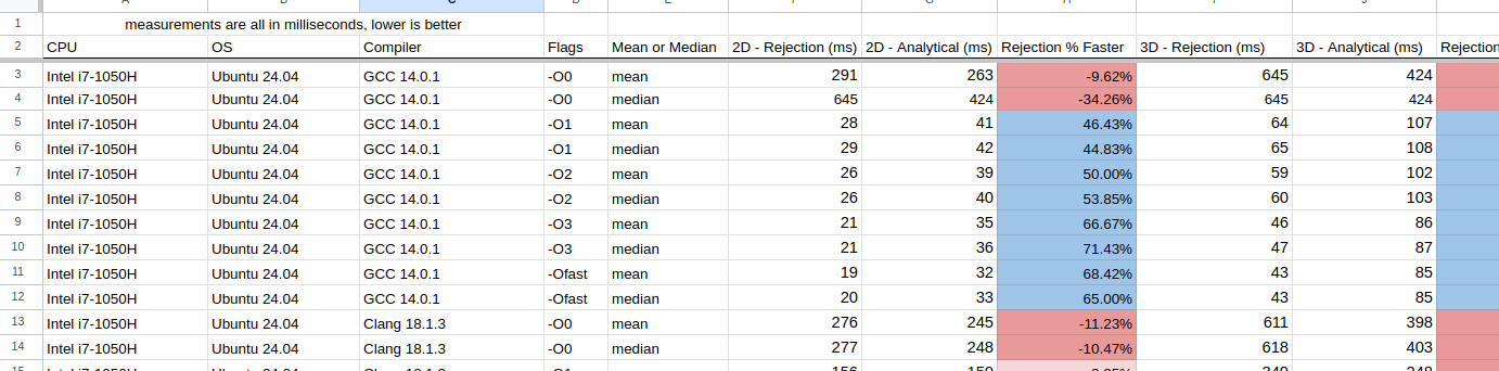
Across these 4 dimensions, there are 48 different combinations and 12 functions to run so that's 576 sets of runs. It... took a while... If you wish to see all of the final data and analysis, it can be found in this Excel sheet and this Jupyter Notebook.

(Data looks like this)

I don't want to bore you with any of the analysis code (see the Jupyter Notebook if you wish).

The key variable in it is ms_faster_treshold = 10.0. So if one style (e.g. "pass by args") is more performant than the other two, that style would need to be at least 10 milliseconds faster.

 

So What Was Discovered?

There isn't much of a difference; barely. Out of those 576 run sets, only a whopping 8 had a significant performance difference. Here are all of them:

A lot of the rows aren't showing a large enough value for the time_ms_faster . Not even single digit improvements, a good chunk being only 0.34 ms or even 0.03 ms faster than the other two; which is not conclusively faster (or slower). Note that a "run set" can take anywhere from 150 ms to 300 ms to complete, which is why we're looking for a speedup of at least 10 ms

So in about 98% of the cases, whether the function was free or a member, had no significant performance difference.

Where there are gains it is (almost) exclusively coming from using clang on x86_64 Linux, at nearly all optimization levels, but only with normalize() where it was a free function using the "pass by args" style. Eyeballing the numbers, it's shaving off ~35 ms from runtimes between 185 ms ~ 205 ms. That is around a ~15% performance increase. It's actually significant! But keep in mind, this is only in 2% of the run sets.

From this benchmark, I think it might be fair to conclude this:

1. Using free functions (with pass by args) can be more performant, but only with specific situations
2. Member vs. free in general doesn't have a performance gain or hit

This was a very limited benchmark; not my favorite. What happens in a larger application?

 

Larger Systems

Small benchmarks are fine, but they can be too "academic" or "clinical". In the sense when they are applied in a bigger program (i.e. "real world"), the results may be vastly different.

As mentioned before the previous posts on this site were concerning my pandemic pet project PSRayTracing. I think it's time to retire it and use something else. Synfig!

If you're wondering "Why Synfig?", let me elaborate:

1. It's another C++ computer graphics (animation!) project
2. It's a bit more "real world practical" than my own ray tracer
3. Fully open source
4. It has a repo of nearly 700 test cases (.sif files)
5. Hacking on it (and around it) is quite easy
6. To automate testing was a sinch

The premise here is we will free a function used in the program and see if it leads to any significant change. The v.1.5.3 release (of Aug 2024) will be the version of code tested.

 

What to Free?

A method that is called a lot.

Freeing one function that is used sparsely makes no sense. I've contributed to the project a very long time ago, but I am not that familiar with the code base so I don't know its ins and outs. It wouldn't be fair to spelunk into the code, grab a random member function, free it, and then do the performance metering. There are tools that exist to find a good candidate.

Callgrind is perfect in our case. For those of you who are unfamiliar, it's part of the Valgrind suite. Its job is to generate call graphs, which can be used to see what functions are being called the most in an application. (Just note that this is very slow to run.)

CMake's build type must be set to RelWithDebInfo. This will compile the application with the -g -O2 flags. -g will add debugging information to the Synfig binaries. And -O2 gives a reasonable level of optimization. The final product would use CMake's Release mode (giving -O3), but we'll go back to that when running the benchmark.

Raw Callgrind output will look like this:

# callgrind format
version: 1
creator: callgrind-3.24.0
pid: 3476
cmd:  /home/ben/Projects/synfig/cmake-build/output/RelWithDebInfo/bin/synfig /home/ben/Projects/synfig-tests/rendering/sources/icons/tool_brush_icon.sif
part: 1

desc: I1 cache: 
desc: D1 cache: 
desc: LL cache: 

desc: Timerange: Basic block 0 - 163286698
desc: Trigger: Program termination

positions: line
events: Ir
summary: 800111840

ob=(235) /usr/lib/x86_64-linux-gnu/libopenmpt.so.0.4.4
fl=(801) ???
fn=(93066) 0x00000000000285a0
0 5

fn=(93056) 0x0000000000028610
0 9
cob=(4) ???
cfi=(179) ???
cfn=(93062) 0x000000000bfdc920
calls=1 0 
0 1292
0 1
cfn=(93066)
calls=1 0 
0 5
0 3

...

368 2
+13 6
cob=(4)
cfi=(179)
cfn=(67574)
calls=1 0  
* 24
fi=(1044)
3235 3
fi=(1045)
381 1
fi=(1044)
3235 1
fe=(1046)
2381 2
fi=(1044)
499 2
fe=(1046)

totals: 800111840

Any output can easily be around 500K lines; I'm cutting a few out for brevity's sake. This seems like a bunch of gibberish, but it needs to be loaded into something like KCachegrind to make some more sense of the output.

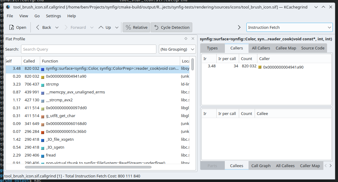
Here we can see this synfig::surface<T>::reader_cook() function is called quite a bit. Maybe it's a good function to free? No. This was only checking a single file, we should be more thorough. Synfig's repo of test data has hundreds of files we can check. An instinct might be to grab a handful of files from this repository and check those. But we can do better: check it all.

Python is amazing. It has everything you need for automating any task. Running Callgrind on a directory tree of 680 files takes a while for a human to do. Python can automate that away for you. So I wrote a script that does that.

The next problem is that we have 680 files containing the Callgrind output. We're not going to load each one of these files in KCachegrind. That would be absurd.

Python is magic. We can easily combine all of this output to make a sort of "merged Callgrind report" from the entire test repo. So I wrote a script that does that.

This uses a slightly different tool by the name of callgrind_annotate, which essentially is a command line version of KCachegrind. It gives us what we need to know: which functions are called the most. Thus letting us hunt down what is the best candidate to free. One thing to note is that there's a lot of non-synfig functions in the callgrind output. For example, if you look at the above screenshot things like strcmp() pops up. We need to filter for only Synfig's code. And that's easily solved via grep:

cat combined_callgrind_output.txt | grep synfig

Which leads us to these candidate functions:

1. CurveGradient::color_func()
2. Color::clamped()
3. bezier::find_closest()

Instead of testing all three, we're only going to test freeing Color::clamped(). It's very simple and what I think is the most straightforward to liberate.

 

How to Free?

There are three different ways we can unbind this function from the Color class:

1. Change it to a friend function
2. Set the data to public
3. Refactor the function to require the caller to pass in arguments
   • this is the proper way

Similar to the smaller benchmark, I don't think there should be any performance difference from the baseline (no changes) to any of the three above methods. friend and public are included here for completeness, despite not being a fully correct freeing technique. I thought it would also be interesting to see if there are any unintended side effects that could affect performance.

 

How to Measure?

We can modify the recursive Callgrind script to instead render all of the sample Synfig files, along with taking down the runtime.

We're going to be more limited though:

1. We'll only keep it to Intel & AMD Linux machines with GCC (14.2)
2. I don't believe building with MSVC works at the moment
3. Building with clang didn't work (see this ticket)
4. We'll only run each file 10 times. As some of the .sif files can take 30+ minutes to render

 

Results & Analysis

Sooo... This also took a while... Just shy of 78 hours. The Jupyter Notebook analysis is here, and the data measurements in this directory.

Altogether the runtimes taken are:

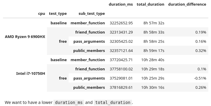
At the surface there are two observations:

1. friend functions and public data members were slightly slower
2. On the Intel CPU, using "pass arguments" (the correct freeing method) was the only one that was actually faster

There is concern though: the percent difference from the baseline is only about half a percent. This isn't significant, it's fair to call this noise. I wouldn't feel confident in saying that free functions were a performance gain or hit here. Taking only 10 samples for each file, we would need to take around 25 before I could feel confident.

We did 10 runs of each Synfig file. What if we took the best runtime for each environment and then totaled that up?

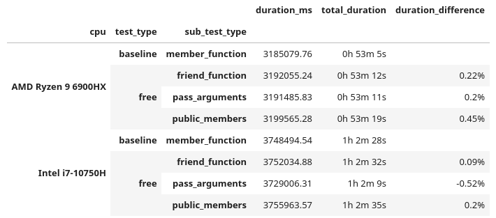
These are similar results, as the duration_difference correlates to the above. But since there is not any significant speedup (beyond 1%), I have to say it's still noise.

Right now we are looking at the cumulative runtime of the entire test repo. What if we found certain test cases that were faster? There is a chance that a specific .sif file could render faster with a free function. Luckily we have all that data to find out if there are any instances where one method was more performant. Applying a minimum 2% faster threshold:

Wow. We have a 44% performance increase for a single case, followed by a bunch of 30% boosts!! That is massive! But... I am a little skeptical. We need to peek into the data. Looking at all of the runtimes for that no. 1 performer:

So... This is a little awkward. Doing 10 runs of each .sif file (for each combination), 9 times we have a measurement of 164 ms, but 1 time it took 114 ms. It doesn't feel right to call that a best case run. I'd call that a bad data point. It's possible there could be some others. Luckily there are ways we can throw out undesirable data. Z-Scores are a way to find outliers:

If we can find them, we can throw them out. Using a threshold of 2.0. This ends up tossing out about 5.3% of the data. Not an ideal, but something that I think we can still work with.

Now this is interesting. When we accumulate all of the runtimes with this cleaned data, each time the free function performs faster than the member function! A few are in the range of noise, but the others are significant. A 1.5% ~ 2.8% speedup! But let's take a look when we filter for the best case runtime:

Now we have a different story. All of the duration differences are back in the range of being noisy. From here, we need to take a deeper look at the (cleaned) data. I took a look at a few of the run sets, finding one in specific that is quite peculiar, no. 754 (which is file 075-ATF-skeleton-group.sif). Computing the Z-scores for this run set:

In these 10 data points:

• Half congregate around 515 ms
• The other half hover at 464 ms
• All of their Z-scores do not go above the threshold (2.0), so each one is kept in
• All of the Z-scores are effectively the value -1.0 and 1.0

This unfortunately means that the entire run set is bad data, which further cascades to the other tests that use the same file, thus requiring us to throw out 80 data points. Not good.

I tried adjusting to have an even more sensitive Z-score threshold (e.g. 1.5, 1.0, etc.) but that led me to throwing out a whooping 30% of the original data. If you play around with the Z-score you will find cases where the free functions were faster, then slower, then faster, then slower... I even tried out IQR as another means of removing bad data, but that also didn't work as desired.

With what we have right now, more testing would be required to make a definitive answer. But for Synfig, I don't find freeing functions concretely helping or hurting performance.

It's also likely that Synfig might not be the best "large integrated benchmark", seeing as we had some files with fluctuating runtimes. Maybe Blender is a better test bed. This is one of the issues of working with a code base you don't know that well. There could be something non-deterministic in the supplied test files. I don't thoroughly know this code; I'm making a wild guess here.

What has been done here is very much in the realm of microbenchmarking. It's hard to do, and difficult to find consistent results.

 

Conclusions & Thoughts on Free Functions

I don't think there is a practical performance benefit.

Architecturally I can see how free functions make sense. But if you're rewriting a function to free it, in hopes that it will make your code faster; it probably will not. It will be a waste of time that could introduce bugs into a working code base. Once again let me remind you, this is an article about nothing.

In the smaller benchmark we did find a significant performance increase, but I need to remind you that it was only being observed 2% of the time and in a very specific case (clang compiled code on Intel/Linux machines). But when we freed a (commonly called) member function in a larger application the performance bounced between being measured as faster or slower, all depending on how we looked at some data.

I don't want to stop others from writing free functions because there are no real performance benefits. I want them to write free functions if they think that is the better solution for their problems. It's very likely back in 2017 when Klaus first gave his talk that free functions were more performant than member functions. From that time to now, it is possible that compilers could have improved to optimize member functions better. As stated before, I'm not familiar with the internals of compilers and their under the hood advancements. I'm a very surface level C++ developer. I have to defer to people smarter than me on this matter.

This is a bit of an aside, but in one of my early jobs I had a higher-on-the-food-chain-coworker who one day wanted everyone to only write code (in Python) using functional paradigms. This was many years ago when Haskell and the ilk were much more in vogue. His claim was "functional programming is less buggy". He never provided any study, research, resource, document, database that backed up this claim. His reasons were vibes and appealing to the authority of Hacker News and that the URL had "medium.com" in it. This paradigm shift did nothing other than just introduce new problems. For example, taking a simple 3 line for-loop and then blowing it up to 7 line indecipherable list comprehension; this happened more than once. If you didn't fall in line, his solution was to berate and shame you in a public Slack channel and ignore your PRs. I'm glad I don't work with this guy anymore.

You might have thought that we proved absolutely nothing here and just wasted a bunch of electricity and time. I've said this twice already. But we've also discovered the inverse: if you want to free a function, you can rest assured there isn't a performance hit. We've also incidentally shown proof that public vs. private data, and friend functions, pass by struct, etc should not cause any performance changes.

I hope that you've watched Klaus' talk, because he does an excellent job of explaining the benefits of free functions. The big one for me is flexibility. I used to dabble in the Nim language a lot more in my past. I still miss it as it's really cute. It has Uniform Function Call Syntax. This makes any language way more ergonomic. Multiple times it has been proposed for C++, and was even talked about in Klaus' presentation. Herb Sutter's Cpp2/cppfront (which I think will be the next major evolution of the language,) has support for UFCS. We will not have any performance hit for this. Give it a try.

My only criticism I have of the old presentation is Klaus never provided a benchmark. I have been watching his talks for years and have always enjoyed them. One of his more recent talks from 2024 does include one. I would like to thank him for taking the time to email me back and forth over the past few months while I worked on this.

If anyone here is also looking for a project to brush up on their C++ skills, Synfig is great to check out. These people were very kind to me years ago when out of nowhere I just plopped in some tiny performance improvements and then didn't return for 5 years. They make it so damn easy to get set up. Blender gets a lot of attention, but I think this project needs some love too.

Since this is now my 4th try investigating performance claims in C++, if anyone has any suggestions on another topic they would like me to investigate, please reach out. I've made lots of scripts and tools in the past year+ to do these investigations. I'm wondering if there is any interest in creating a generic tool to do performance metering and test verification. I want to take a break and work on other projects in the near future though. So I won't be doing anything like this for a while.

Likewise, if anyone is interested in me profiling/investigating the performance of their code, reach out as well.

My main hope is that with these articles, we will stop making claims (i.e. performance improvements) without providing any measurements to back up our statements. We're making wild assertions but not testing them. This needs to stop.

If you just scrolled down here for the tl;dr: free functions don't have much of any performance difference from that of member functions.

/r/cpp discussion thread here.

Update February 16th, 2025:  I've posted this article on a few places, and if you've read the comments sections (such as on /r/cpp), it's well mentioned that this was very poorly titled.  I would like to acknowledge this fact.  The title was not my number one priority when writing this post; the content was.  With this said, I'm not going to be changing anything below.

1. I'd need to change many URLs and possibly break linkage to this.  That's a lot of work
2. We all goof up at times.  I don't want to hide this and would like to show to our more junior developers that your seniors will make mistakes as well
3. /u/STL was generous enough to bestow a custom post flair on the article



Those aren't handed out to just anyone.  You have to work for that, and hard.

In the realm of computer science, we're always told to pursue what is the most efficient solution. This can be either what is the fastest way to solve a problem; or what may be the cheapest.

What is the easiest, but not always the best, is typically a "greedy algorithm"; think bubble sort. More often than not, there is a much more efficient method which typically involves thinking about the problem a bit deeper. These are often the analytical solutions.

Whilst working on PSRayTracing (PSRT), I was constantly finding inefficient algorithms and data structures. There are places where it was obvious to improve something, whereas other sections really needed a hard look-at to see if there was more performance that could be squeezed out. After the podcast interview I was looking for the next topic to cover. Scanning over older code, I looked at the random number generator since it's used quite a bit. I spotted an infinite loop and thought "there has to be something better".

The code in question is a method to generate a 2D (or 3D) vector, which falls within a unit circle (or sphere). This is the algorithm that the book originally gave us:

Vec3 get_in_unit_disk() {
    while (true) {
        const Vec3 p(get_real(-1, 1), get_real(-1, 1), 0);
        if (p.length_squared() >= 1)
            continue;

        return p;
    }
}

The above in a nutshell:

1. Generate two (random) numbers between [-1.0, 1.0] to make a (2D) vector
2. If the length squared of the vector is 1 or greater, do step 1 again
3. If not, then you have a vector that's within the unit circle

(The 3D case is covered by generating three numbers at step 1)

 

This algorithm didn't feel right to me. It has some of that yucky stuff we hate: infinite looping and try-and-see-if-it-works logic. This could easily lead to branch prediction misses, being stuck (theoretically) spinning forever, wasting our random numbers. And it doesn't feel "mathematically elegant".

My code had some commented out blocks with an analytical solution to the above. But in the years prior when I had first touched that code I had left a note saying that it was a bit slower than using the loop.

The next day I had an email fall into my inbox. It was from GitHub notifying me of a response. The body was about how to generate a random point inside of a unit sphere... Following the link to the discussion, it came from the original book's repository. The first reply in 4 years on a topic... that... I... created...

I think this was a sign from above to investigate it again.

 

Reading through the old discussion ^{(please don't look I'm embarrassed)}, one of the maintainers @hollasch left a good comment:

What really stuck out to me is in the beginning:

"The current approach is significantly faster in almost all cases than any analytical method so far proposed ... every time our random sampling returns an answer faster than the analytical approach,"

Are rejection methods much faster than an analytical solution? Huh.

 

Understanding The Problem A Little More

As seen above, there is an analytical solution to the above algorithm for both the 2D and 3D cases. We'll use Python for the moment.

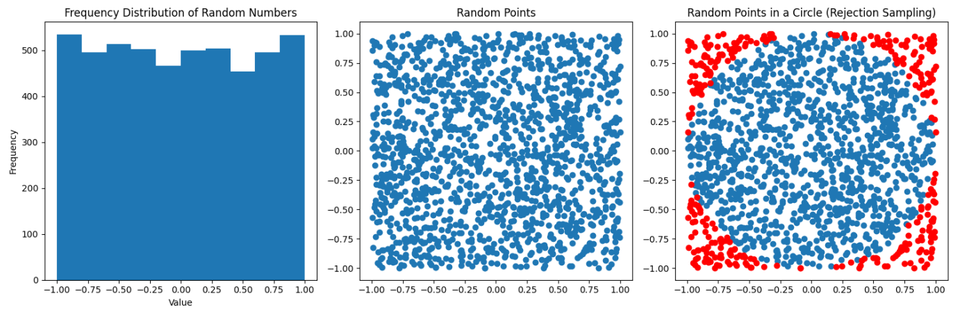
In the above diagrams, we're just taking a random sampling of points inside a 2D plane. You can see they are fairly uniformly distributed. To the far right the points in blue are what falls within the unit circle, the red is what falls outside (and we must throw out). In a nutshell this is a visualization of the rejection sampling method:

def rejection_in_unit_disk():
   while True:
       x = random.uniform(-1, 1)
       y = random.uniform(-1, 1)
       v = Vec2(x, y)

       if (v.length_squared() < 1):
           return v

 

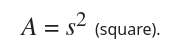
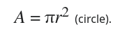
Using the area formulas for a square and a circle, we can find out the chance that a point will fall inside the circle:

In this case, r = s / 2, and it's <circle area> / <square area>. If you do all of the math, you'll find that the odds are ~78.54%. Which means that around 22% of our points are rejected; that isn't desirable.

For the analytical solution, you have to think in terms of polar coordinates: Generate a random radius and generate a random angle. Initially you might assume the correct method is this:

def analytical_in_unit_disk_incorrect():
   r = random.uniform(0, 1)
   theta = random.uniform(0, two_pi)
   x = r * math.cos(theta)
   y = r * math.sin(theta)

   return Vec2(x, y)

 

But that's not quite right:

 

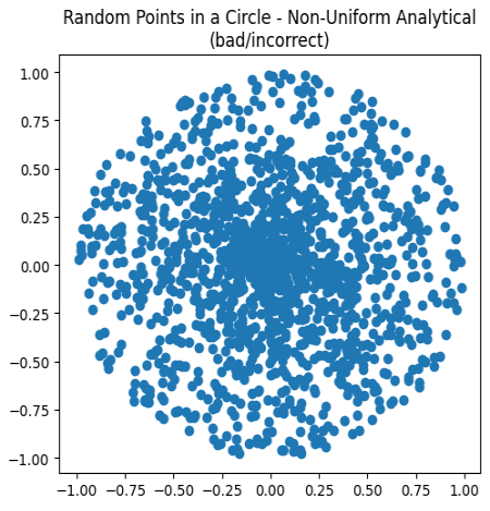
Charting these points, while all are falling within the unit circle, they are clustering more in the center. This is not correct. We need to alter the distribution of the points to appear more uniform. Remember from math class how you needed to use a square root to calculate the distance of a vector? That's also the trick to fixing the scattering:

def analytical_in_unit_disk():
   r = math.sqrt(random.uniform(0, 1))
   theta = random.uniform(0, two_pi)
   x = r * math.cos(theta)
   y = r * math.sin(theta)

   return Vec2(x, y)

 

Huzzah! We now have the analytical solution:

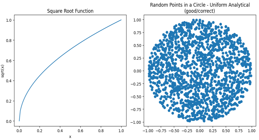
Look at how beautiful that is:

1. All points fall within the unit circle
2. All look to be equally distributed
3. No (theoretical) infinite looping
4. No wasted random numbers

The 3D case the rejection method is the same (but you add an extra Z-axis).

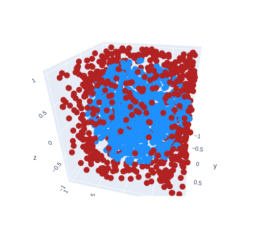
How much more inefficient is the rejection sampling in 3D? It's way worse than the 2D case. Take these volume formulas. The first being that of a cube's and the second that of a sphere's.

Similarly, when a = r / 2, the chance a randomly generated point (using rejection sampling) falls within the sphere, is only 52.36%. You have to throw out nearly half of your points!

The analytical (spherical) method is a tad more complex, but it follows the same logic. If you want to read more about this, Karthik Karanth wrote an excellent article. The Python code for the 3D analytical solution is as follows:

def analytical_in_unit_sphere():
   r = math.cbrt(random.uniform(0, 1))
   theta = random.uniform(0, two_pi)
   phi = math.acos(random.uniform(-1, 1))

   sin_theta = math.sin(theta)
   cos_theta = math.cos(theta)
   sin_phi = math.sin(phi)
   cos_phi = math.cos(phi)

   x = r * sin_phi * cos_theta
   y = r * sin_phi * sin_theta
   z = r * cos_phi

   return Vec3(x, y, z)

 

Jumping ahead in time just a little, let me show you the same scene rendered twice over, but with each different sampling method:

 

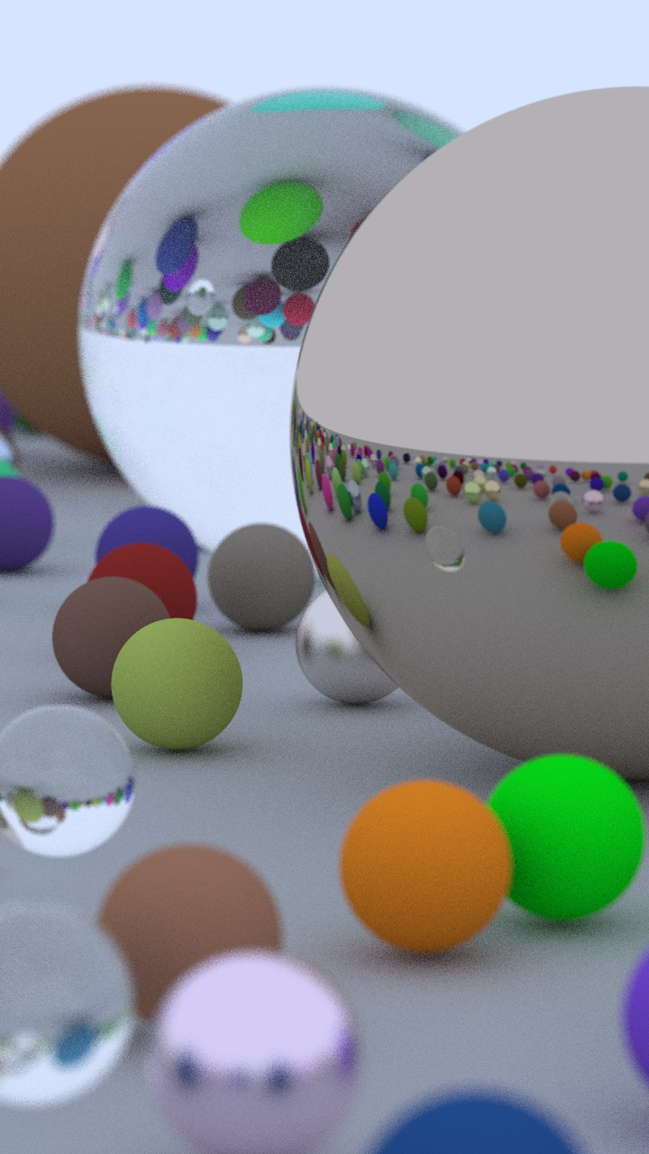
The one on the left was using boring rejection sampling, whereas the one on the right is using this new fancy analytical method. At a first glance the two images are indistinguishable; we'd call this "perceptually the same". Zooming in on a 32x32 patch of pixels (in the same location) you can start to spot some differences.  This is because we are now traversing through our random number generator differently with these two methods.  It alters the fuzz, but for the end user it is the same image.

_{(Hint: look at the top two rows, especially the purple near the right side)}

 

Benchmarking (Part 1)

Let's stay in Python land for the moment because it's easier. We can create a small benchmark to see how long it takes to generate both the 2D & 3D points. The full source code of the program can be found here. The critical section is this:

# Returns how many seconds it took
def measure(rng_seed, num_points, method):
   bucket = [None] * num_points  # preallocate space

   random.seed(rng_seed)

   start_time = time.time()
   for i in range(0, num_points):
       bucket[i] = method()
   end_time = time.time()

   return (end_time - start_time)


def main():
   rng_seed = 1337
   num_runs = 500
   num_points = 1000000

   # ...

   for i in range(0, num_runs):
       seed = rng_seed + i

       r2d = measure(seed, num_points, rejection_in_unit_disk)
       a2d = measure(seed, num_points, analytical_in_unit_disk)
       r3d = measure(seed, num_points, rejection_in_unit_sphere)
       a3d = measure(seed, num_points, analytical_in_unit_sphere)

       # ...

 

From there we can take measurements of how long each method took and compare them. Running on a 10th Gen i7 (under Linux), this is the final runtime of the benchmark:

Rejection 2D:
  Mean: 0.893 s
  Median: 0.893 s
Analytical 2D:
  Mean: 0.785 s
  Median: 0.786 s
Rejection 3D:
  Mean: 1.559 s
  Median: 1.560 s
Analytical 3D:
  Mean: 1.151 s
  Median: 1.150 s

 

Looking at the median rejection sampling is 13% slower in the 2D case and 35% in the 3D case!! Surely, we must now use the analytical method. All of this work we've done was definitely worth it!

 

Taking It Into The Ray Tracer

Placing the analytical methods into the ray tracer was very trivial. All of the math functions exist in the standard library therefore the port from Python is nearly 1-1 one to one. Here's how long it takes to the render the default scene with the sad-poor rejection sampling:

me@machine:$ ./PSRayTracing -j 4 -n 500 -o with_rejection.png
...
Render took 105.956 seconds

 

And now, recompiled with our Supreme analytical method:

me@machine:$ ./PSRayTracing -j 4 -n 500 -o with_analytical.png
...
Render took 118.408 seconds

^{(These measurements were taken with the same 10th Gen i7 on Linux compiled with GCC 14 using CMake's Release mode.)}

Wait, it took longer to use the analytical method?  Inspecting both renders they are perceptually the same. Pixel for pixel there are differences, but this is expected because the random number generator is being used differently now.

Just like my note from 4 years ago said... It's... Slower... Something Ain't Right.

 

Benchmarking (Part 2)

We need to dig in a little more here. Let's benchmark the four methods separate from the ray tracer again, but this time in C++. If you want to read the source, I'll leave the link right here: comparing_greedy_vs_analytical.cpp . It's structured a tiny bit different from the Python code, but we have as little overhead as possible. We'll also be using the same RNG engine, the Mersenne Twister (MT).

I want to take an aside here to mention that PSRT actually uses PCG by default for random number generation. It's much more performant than the built in MT engine and doesn't get exhausted as quickly. I wrote about it briefly before. The MT engine can be swapped back in if so desired. While any random number generation method can greatly impact performance, in this case it is not the cause of the slowdown seen above.

me@machine:$ g++ comparing_greedy_vs_analytical.cpp -o test
./test 1337 500 1000000
Testing with 1000000 points, 500 times...
run_number: rejection_2d_ms, analytical_2d_ms, rejection_3d_ms, analytical_3d_ms
1: 516, 268, 658, 423,
2: 295, 273, 640, 428,
...
499: 306, 278, 670, 445,
500: 305, 279, 676, 446,

mean: 313, 277, 675, 448
median: 305, 276, 665, 444
(all times measured are in milliseconds)

 

It's still showing the analytical method is still much more faster than the rejection sampling. About 10% for 2D and nearly 33% for 3D. Which is what is aligned with the Python benchmark. What could be going on here...  Oh wait; Silly me...

I forgot to turn on compiler optimizations... Let's run this again now!

me@machine:$ g++ comparing_greedy_vs_analytical.cpp -o test -O3
./test 1337 500 1000000
Testing with 1000000 points, 500 times...
run_number: rejection_2d_ms, analytical_2d_ms, rejection_3d_ms, analytical_3d_ms
1: 87, 137, 96, 81,  
2: 17, 33, 40, 80,  
...
499: 18, 35, 42, 82,  
500: 18, 35, 44, 82,  

mean: 20, 38, 44, 82
median: 17, 34, 42, 82
(all times measured are in milliseconds)

 

What-

The rejection sampling methods are faster?! And by 50%?!!?!

This needs more investigation.

 

Benchmarking (Part 3)

If you've read the other posts in this series, you know that I like to test things on every possible permutation/combination that I can think of.  At my disposal, I have:

• An Intel i7-1050H
• An AMD Ryzen 9 6900HX
• An Apple M1

With the x86_64 processors I can test GCC, clang, and MSVC. GCC+Clang on Linux and GCC+MSVC on Windows. For macOS we're playing with ARM processors so I only have Clang+GCC available. This gives us 10 different combinations of Chip+OS+Compiler to measure. But seeing above how optimizations levels affected the runtime we need to look at different compiler optimization flags (-O1, -Ofast, /Od, /Ox, etc). In total there are 48 cases which can be tested.

 

Using the above C++ benchmark, the results have been placed into a Google Sheet. As always, they yield some fascinating results:

Normally, I would include some fancy charts and graphs here, but I found it very difficult to do so and I didn't want to cause any confusion. Instead there are some interesting observations I want to note:

• For Intel+Linux+GCC just turning on -O1 yielded significant improvements
  • On average, optimizations made rejection sampling 50% faster
• For Intel+Linux+Clang in nearly all of the cases, the analytical method was faster
  • Especially for 3D
  • The only exception was when -Ofast was used, the rejection sampling performed better
• For Intel+Windows+GCC rejection sampling was always better. Typically +150% for the 2D case, and +70% for 3D
• Intel+Windows+MSVC is comparable to the above (GCC) but was slower
• On AMD, all compilers on each OS behaved the same as on Intel
• With the M1 chip (macOS) GCC performed much better than clang
  • Except for -O0 GCC's rejection sampling was always faster than the analytical method
  • Clang on the other hand, 2D rejection sampling was faster, but for the 3D case, using the analytical method was faster.

This is a bit bonkers, as I really didn't expect there to be that much difference. Clang seemed to do better with analytical sampling, but GCC (with optimizations on) using rejection sampling stole the show. In general, I'm going to claim now that rejection sampling is better to use.

 

Assembly Inspection

I'm always iffy when it comes to inspecting the assembly. It's not my wheelhouse, and playing "count the instructions" is my favorite way of measuring performance; running code with a stopwatch is. If you need a basic primer on the topic, these two videos give a nice overview about some more of the important parts:

• x86_64 jumps and control flow
• X86_64 calls

Reducing instruction counts, jumps and calls are what we aim for.

Taking a look at GCC 14.2's x86_64 output, the -O0 case is quite straightforward. We're going to only cover the 2D case as it's less to go through.

First up with rejection sampling (full code here), it will take around ~110 instructions to fully complete. Coupled with that we have 4 procedure calls and at the end a check to see if we need to repeat the entire process (and remember there is 22% chance it could happen). In the case we repeat it, then it would be around ~205 instructions (and 8 procedure calls).

In the analytical case (full code here) there's a little less than ~100 instructions to compute. Now on the flip-side there are 6 calls, but there is zero chance that we'll have to repeat anything in the procedure.

When cracking up that compiler to -O3, we have to throw everything above out the window as the assembly becomes very hard to decipher. I'll try my best, but if I'm wrong, someone who could contact me to correct it would be much appreciated

(Full code here) This is where I think the rejection method is in the code. This is because of the jne L16 line. A similar pattern of execution is viewed above for -O0. The compiler is optimizing away and inlining a bunch of other functions which makes this hard to track. Here, we have only 45 instructions to run, and not a single call!

(Full code here) This is my best guess of the -O3'd analytical method. The clue here for us is there are the two call instructions; one to sincos() and sqrt(). This looks to be about 55 instructions long, which already loses the counting competition. Coupled in with the calls this will definitely be slower.

Measuring the runtime of the code will always beat looking at assembly. The assembly can give you insights, but it's worthless in the face of a clock. And as you can see from turning on -O3 (or even -O1) it can be much harder to glean anything useful.

 

Benchmarking (Part 4)

Just because the smaller test case shows a 50%+ performance boost in some cases, that doesn't mean we'll see that same increase in the larger application. A benchmark of a small piece of code is meaningless until it's been placed into a larger application. If you've read the previous posts from this blog, this is where I like to do some exhaustive testing of the Ray Tracing code for hundreds of hours. 🫠🫠🫠

The testing methodology is simple:

1. There are 20 scenes in the ray tracer
2. We'll test each of them 50 times over with different parameters
3. The same test will be run once with rejection sampling and once with the analytical method
4. The difference in runtime will be written down

I need to note I turned on the use of the real trig functions this time. By default PSRT will use (slightly faster) trig approximations. But to better keep in line with the benchmark from above, 100% authentic-free-range-organic-gluten-free-locally-grown sin(), cos(), atan2(), etc() was used. You can read more about the approximations here.

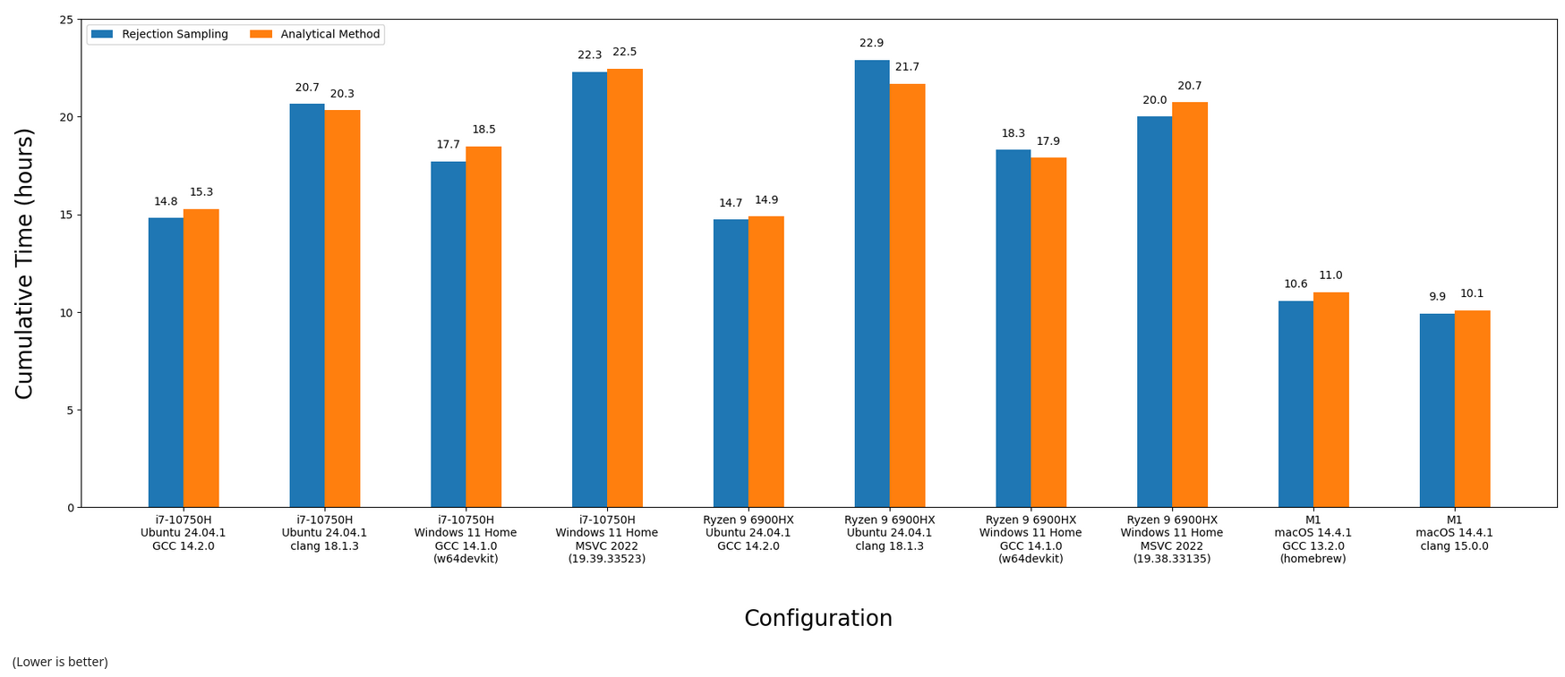
After melting all of the CPUs available to me, here are the final results. Everything was compiled in (CMake's) Release mode, which should give us the fastest code possible (e.g. -O3):

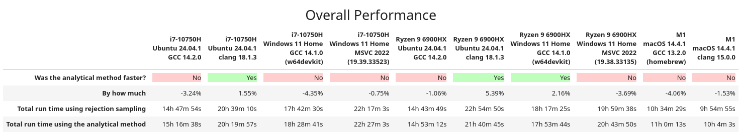
In some cases, rejection sampling was faster, in others using the analytical method was. Visualizing the above as fancy bar charts:

 

 

The scene by scene breakdown is more intriguing. Here's the means and medians for each scene vs. configuration:

 

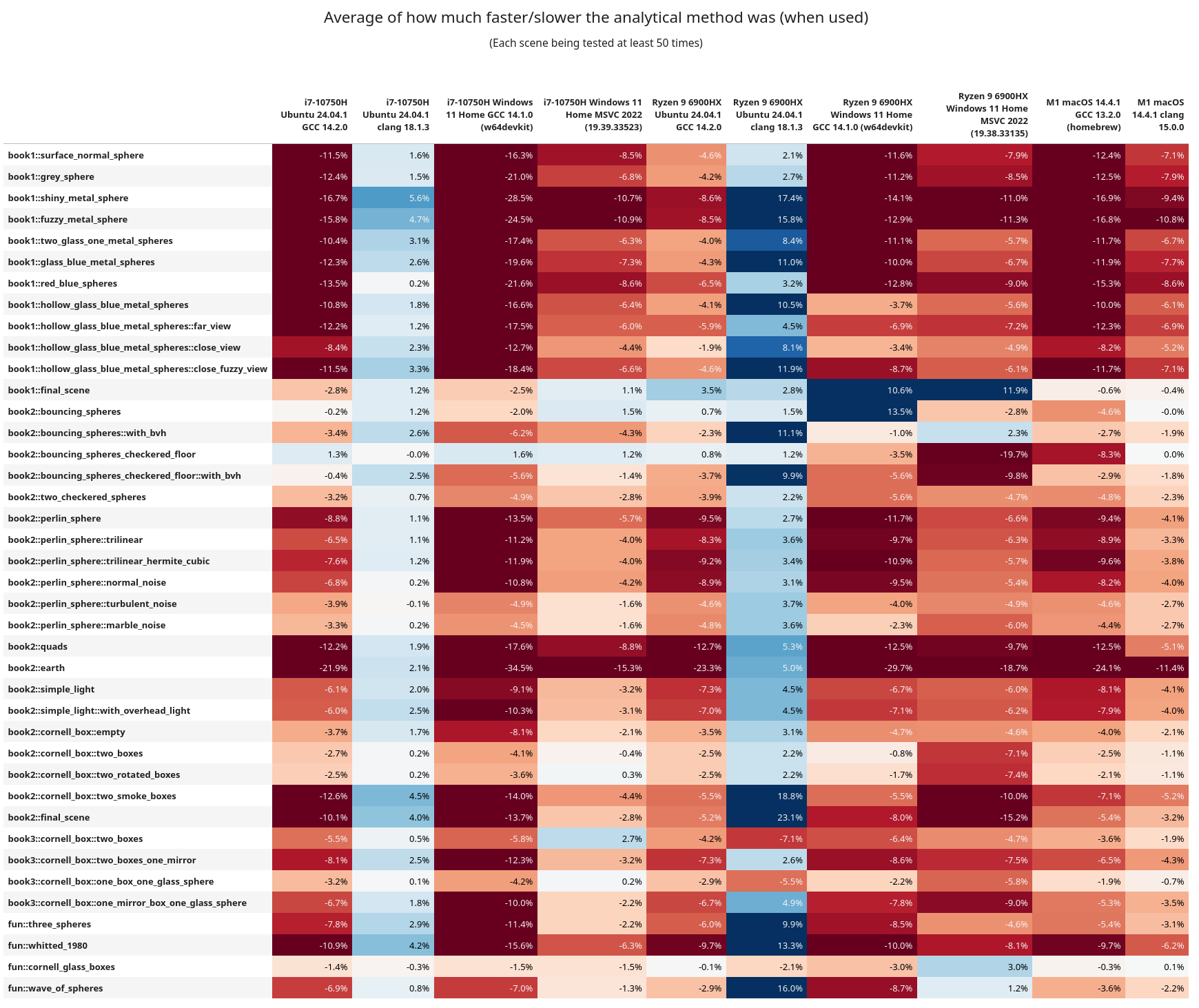
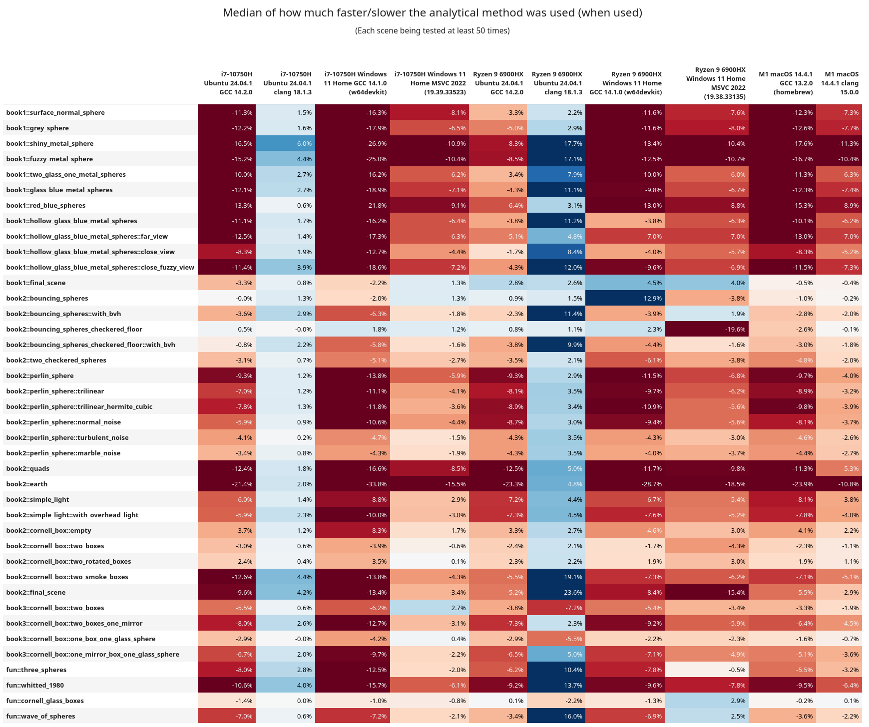
Here are some of the interesting observations:

• In general, rejection sampling is MUCH more performant, and sometimes by a wide margin
• Clang was having a better time on x86_64 when using the analytical method
  • But keep in mind GCC is overall more performant, and with rejection sampling instead
• book1::final_scene and book2::bouncing_spheres have lots of elements in them, but are not using a BVH tree for ray traversal. Across the board rejection sampling isn't helping too much, and in fact the analytical method is more performant.
• After them these scenes have a with_bvh variant (that does use the BVH tree) and they then see a benefit from rejection sampling.
  • When using analytical sampling the AMD chip isn't getting hit as hard on performance as the Intel one. This is more easily observed in the book1 scenes.  Following these, all of the scenes now use a BVH tree
  • On Linux+GCC, Intel and AMD ran the entire test suite in approximately the same time, but AMD was every so slightly faster
  • Linux+Clang ran better on Intel
  • Intel+Windows+GCC had rejection faster, but AMD+Windows+GCC did better with analytical
  • AMD ran the Windows+MSVC code significantly faster (by 2 hours!!)
  • From the assembly inspection above, I wonder if maybe the AMD chips are better at running the call instruction? Or are better at running some of the math functions. This is wild guessing at this point.
  • I do want to note that these are chips from different generations, so it can be like comparing apples to oranges.

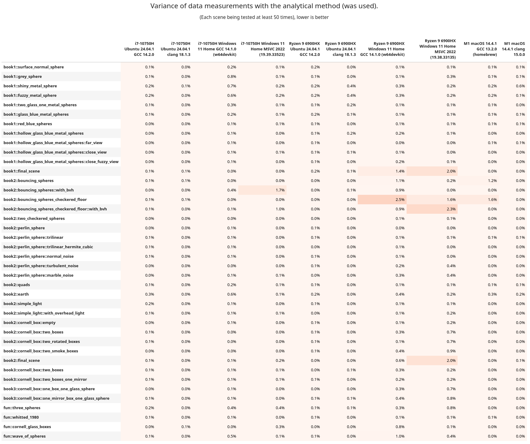
If you want to see the variance from the above tables, it's here, but it's more boring to look at.

 

Benchmarking (Part 5)

While clang was slower than GCC, it was surprising to see that it actually had a performance benefit when running the analytical method. Seeing how Python also fared better with this method, I thought it might be worth seeing what happens elsewhere. Clang is built upon LLVM, So it's possible that this could have an effect on other languages of that lineage. Let's take a trip to the Rustbelt.

To keep things as simple as possible, we're going to port the smaller C++ benchmark (not PSRT). I've tried to keep it as one-to-one as possible too. The code is nothing special, so I'll link it right here if you wish to take a look. This is the first Rust program I have ever written; please be gentle.

Running on the same Intel & Linux machine as above (using rustc v1.83), Debug (no optimizations) reported that rejection was slower and the analytical faster:

Testing with 1000000 points, 500 runs...    [rng_seed=1337]
run number: rejection_2d_ms, analytical_2d_ms, rejection_3d_ms, analytical_3d_ms
1: 216, 202, 480, 344
2: 218, 206, 475, 344
...
499: 210, 198, 454, 329
500: 209, 198, 454, 328

mean: 211, 199, 459, 332
median: 211, 199, 458, 331
(all times are measured in milliseconds)

 

And with Release turned on rejection was faster:

Testing with 1000000 points, 500 runs...    [rng_seed=1337]
run number: rejection_2d_ms, analytical_2d_ms, rejection_3d_ms, analytical_3d_ms
1: 24, 32, 49, 81
2: 19, 32, 44, 82
...
499: 19, 32, 44, 82
500: 19, 32, 44, 81

mean: 19, 31, 43, 81
median: 19, 32, 44, 82
(all times are measured in milliseconds)

 

What's fun to note here is this Rust version is slightly faster than its C++/GCC equivalent. But when the same code is compiled with C++/Clang it doesn't do as well (check rows 11, 12, 21, & 22).  I'm glad to see that Rust is exhibiting the same behavior as C++ with and without optimizations.

 

Closing Remarks

After all of this work, PSRT will stick with using the naive rejection sampling over the beautiful analytical method. It's frustrating to spend time on something you thought was the better way, only to find out that, well, it isn't.

If there is one main take away from this post: always test and measure your code. Never trust, only test. Unexpected things may happen, and results may change over time. It's the same thing I've been saying since the first article. And it bears repeating because not enough people do this. You can inspect assembly, reduce branches, get rid of loops, use faster RNGs, etc. But all of that can go out the window if runtime was never recorded and compared.

Remember, the compiler will always be smarter than you and optimizations are wizard magic that we don't deserve.

 

This past week I was invited onto CppCast (episode 389) to talk about some of the C++ language benchmarking I've been doing and about PSRayTracing a little bit too.  I'd like to thank Phil Nash and Timur Doumler for having me on.